Summary of Lecture 6 𝐄 𝐄 𝐀 ( a , b ) \mathbf{EEA}(a, b) input a , b ( a ≥ b > 0 ) a, b\,(a \ge b > 0) output d = gcd ( a , b ) d = \gcd(a, b) s , t s, t d = a s + b t d = as + bt
r 0 = a ; r 1 = b ; ( s 0 t 0 ) = ( 1 0 ) ; ( s 1 t 1 ) = ( 0 1 ) ; r_0 = a; r_1 = b; \begin{pmatrix} s_0 \\ t_0 \end{pmatrix} = \begin{pmatrix} 1 \\ 0 \end{pmatrix}; \begin{pmatrix} s_1 \\ t_1 \end{pmatrix} = \begin{pmatrix} 0 \\ 1 \end{pmatrix}; r 0 = r 1 q 1 + r 2 ( 0 < r 2 < r 1 ) ; ( s 2 t 2 ) = ( s 0 t 0 ) − q 1 ( s 1 t 1 ) r_0 = r_1q_1 + r_2\,(0 < r_2 < r_1); \begin{pmatrix} s_2 \\ t_2 \end{pmatrix} = \begin{pmatrix} s_0 \\ t_0 \end{pmatrix} – q_1 \begin{pmatrix} s_1 \\ t_1 \end{pmatrix} ⋮ \vdots r i − 1 = r i q i + r i + 1 ( 0 < r i + 1 < r i ) ; ( s i + 1 t i + 1 ) = ( s i − 1 t i − 1 ) − q i ( s i t i ) r_{i-1} = r_iq_i + r_{i+1}\,(0 < r_{i+1} < r_i); \begin{pmatrix} s_{i+1} \\ t_{i+1} \end{pmatrix} = \begin{pmatrix} s_{i-1} \\ t_{i-1} \end{pmatrix} – q_i \begin{pmatrix} s_i \\ t_i \end{pmatrix} ⋮ \vdots r k − 2 = r k − 1 q k − 1 + r k ( 0 < r k < r k − 1 ) ; ( s k t k ) = ( s k − 2 t k − 2 ) − q k − 1 ( s k − 1 t k − 1 ) r_{k-2} = r_{k-1}q_{k-1} + r_k\,(0 < r_k < r_{k-1}); \begin{pmatrix} s_k \\ t_k \end{pmatrix} = \begin{pmatrix} s_{k-2} \\ t_{k-2} \end{pmatrix} – q_{k-1} \begin{pmatrix} s_{k-1} \\ t_{k-1} \end{pmatrix} r k − 1 = r k q k r_{k-1} = r_kq_k output r k , s k , t k r_k, s_k, t_k O ( ℓ ( a ) ℓ ( b ) ) O(\ell(a)\ell(b))
Notations: Ω , Θ , π ( x ) = ∑ p ≤ x 1 , v p ( n ) \Omega, \Theta, \pi(x) = \sum_{p \le x} 1, v_p(n) p v p ( n ) | n , p v p ( n ) + 1 ∤ n p^{v_p(n)} | n, p^{v_p(n)+1} \nmid n
THEOREM (Chebyshev, 1850) π ( x ) = Θ ( x ln x ) \pi(x) = \Theta\left(\frac{x}{\ln x}\right)
LEMMA: Suppose that m ∈ ℤ + m \in \mathbb{Z}^+
( 2 m m ) ≥ 2 2 m 2 m and ( 2 m + 1 m ) ≤ 2 2 m \binom{2m}{m} \ge \frac{2^{2m}}{2m} \text{ and } \binom{2m+1}{m} \le 2^{2m} LEMMA: Suppose that p p n ∈ ℤ + n \in \mathbb{Z}^+
v p ( n ! ) = ∑ k ≥ 1 ⌊ n / p k ⌋ v_p(n!) = \sum_{k \ge 1} \lfloor n/p^k \rfloor THEOREM: Let n ∈ ℤ + n \in \mathbb{Z}^+ n ≥ 2 n \ge 2 π ( n ) ≥ ln 2 2 ⋅ n ln n \pi(n) \ge \frac{\ln 2}{2} \cdot \frac{n}{\ln n}
COROLLARY: π ( x ) = Ω ( x ln x ) \pi(x) = \Omega\left(\frac{x}{\ln x}\right) π ( x ) ≥ ln 2 4 ⋅ x ln x \pi(x) \ge \frac{\ln 2}{4} \cdot \frac{x}{\ln x}
Chebyshev’s Theorem COROLLARY: π ( x ) = Ω ( x ln x ) \pi(x) = \Omega\left(\frac{x}{\ln x}\right)
For any real number x ≥ 2 x \ge 2 π ( x ) ≥ π ( ⌊ x ⌋ ) ≥ ln 2 2 ⋅ ⌊ x ⌋ ln ⌊ x ⌋ ≥ ln 2 2 ⋅ x − 1 ln x ≥ ln 2 4 ⋅ x ln x \pi(x) \ge \pi(\lfloor x \rfloor) \ge \frac{\ln 2}{2} \cdot \frac{\lfloor x \rfloor}{\ln \lfloor x \rfloor} \ge \frac{\ln 2}{2} \cdot \frac{x-1}{\ln x} \ge \frac{\ln 2}{4} \cdot \frac{x}{\ln x} Chebyshev’s theta function: θ ( x ) = ∑ p ≤ x ln p \theta(x) = \sum_{p \le x} \ln p // θ ( 5.2 ) = ln 2 + ln 3 + ln 5 = ln 30 \theta(5.2) = \ln 2 + \ln 3 + \ln 5 = \ln 30
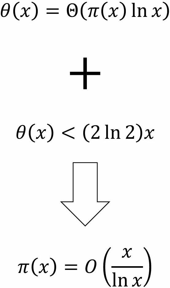
THEOREM: θ ( x ) = Θ ( π ( x ) ln x ) \theta(x) = \Theta(\pi(x) \ln x)
θ ( x ) ≤ π ( x ) ⋅ ln x \theta(x) \le \pi(x) \cdot \ln x // there are π ( x ) \pi(x) terms in θ ( x ) \theta(x) , each of which is ≤ ln x \le \ln x θ ( x ) ≥ ∑ x < p ≤ x ln p \theta(x) \ge \sum_{\sqrt{x} < p \le x} \ln p ≥ ( π ( x ) − x ) ln x \ge (\pi(x) – \sqrt{x}) \ln \sqrt{x} // there are at least π ( x ) − x \pi(x) – \sqrt{x} terms in the sum ∑ x < p ≤ x ln p \sum_{\sqrt{x} < p \le x} \ln p , each ≥ ln x \ge \ln \sqrt{x} = 1 2 ( 1 − x π ( x ) ) π ( x ) ln x = \frac{1}{2} \left( 1 – \frac{\sqrt{x}}{\pi(x)} \right) \pi(x) \ln x π ( x ) ≥ ln 2 4 ⋅ x ln x ⇒ x π ( x ) ≤ 4 ln x x ln 2 → 0 \pi(x) \ge \frac{\ln 2}{4} \cdot \frac{x}{\ln x} \Rightarrow \frac{\sqrt{x}}{\pi(x)} \le \frac{4 \ln x}{\sqrt{x} \ln 2} \to 0 x → ∞ x \to \infty x π ( x ) < 1 2 \frac{\sqrt{x}}{\pi(x)} < \frac{1}{2} x x x ≥ x 0 x \ge x_0 θ ( x ) ≥ 1 4 π ( x ) ln x \theta(x) \ge \frac{1}{4} \pi(x) \ln x x ≥ x 0 x \ge x_0 THEOREM: For any integer n ≥ 1 , θ ( n ) < ( 2 ln 2 ) n n \ge 1, \theta(n) < (2 \ln 2)n
n = 1 : θ ( 1 ) = 0 < ( 2 ln 2 ) ⋅ 1 n = 1: \theta(1) = 0 < (2 \ln 2) \cdot 1 n = 2 : θ ( 2 ) = ln 2 < ( 2 ln 2 ) ⋅ 2 n = 2: \theta(2) = \ln 2 < (2 \ln 2) \cdot 2 n = 3 : θ ( 3 ) = ln 2 + ln 3 < ( 2 ln 2 ) ⋅ 3 n = 3: \theta(3) = \ln 2 + \ln 3 < (2 \ln 2) \cdot 3 ln 6 < ln 2 6 \ln 6 < \ln 2^6 n > 3 n > 3 2 | n 2|n θ ( n ) = θ ( n − 1 ) < ( 2 ln 2 ) ( n − 1 ) < ( 2 ln 2 ) n \theta(n) = \theta(n-1) < (2 \ln 2)(n-1) < (2 \ln 2)n n > 3 n > 3 2 ∤ n 2 \nmid n m ≥ 2 m \ge 2 n = 2 m + 1 n = 2m + 1 M = ( 2 m + 1 m ) = ( 2 m + 1 ) ⋯ ( m + 2 ) m ! < 2 2 m M = \binom{2m+1}{m} = \frac{(2m+1)\cdots(m+2)}{m!} < 2^{2m} Any prime p , m + 1 < p ≤ 2 m + 1 p, m+1 < p \le 2m+1 M M θ ( 2 m + 1 ) − θ ( m + 1 ) = ∑ m + 1 < p ≤ 2 m + 1 ln p \theta(2m+1) – \theta(m+1) = \sum_{m+1 < p \le 2m+1} \ln p ≤ ln M \le \ln M < ( 2 ln 2 ) m < (2 \ln 2)m θ ( n ) = θ ( 2 m + 1 ) − θ ( m + 1 ) + θ ( m + 1 ) \theta(n) = \theta(2m+1) – \theta(m+1) + \theta(m+1) < ( 2 ln 2 ) m + ( 2 ln 2 ) ( m + 1 ) < (2 \ln 2)m + (2 \ln 2)(m+1) = ( 2 ln 2 ) n = (2 \ln 2)n THEOREM: For any real number x ≥ 1 , θ ( x ) < ( 2 ln 2 ) x x \ge 1, \theta(x) < (2 \ln 2)x θ ( x ) = θ ( ⌊ x ⌋ ) < ( 2 ln 2 ) ⌊ x ⌋ < ( 2 ln 2 ) x \theta(x) = \theta(\lfloor x \rfloor) < (2 \ln 2)\lfloor x \rfloor < (2 \ln 2)x
Prime Number Theorem DEFINITION: For x ∈ ℝ + x \in \mathbb{R}^+ π ( x ) = ∑ p ≤ x 1 \pi(x) = \sum_{p \le x} 1 # \# ≤ x \le x
THEOREM (Hadamard;Poussin,1896) lim x → ∞ π ( x ) x ln x = 1 \lim_{x \to \infty} \frac{\pi(x)}{\frac{x}{\ln x}} = 1
Conjectured by Legendre and Gauss (1777-1855) in 1791, proved independently by Hadamard (1865-1963) and de la Vallée Poussin (1866-1962) in 1896 Chebyshev: if the limit exists, then it is equal to 1 1 Rosser (1907-1989) and Schoenfeld (1920-2002) proved in 1962:π ( x ) > x ln x ( 1 + 1 2 ln x ) \pi(x) > \frac{x}{\ln x} (1 + \frac{1}{2 \ln x}) x ≥ 59 x \ge 59 π ( x ) < x ln x ( 1 + 3 2 ln x ) \pi(x) < \frac{x}{\ln x} (1 + \frac{3}{2 \ln x}) x > 1 x > 1 NOTATION: ℙ \mathbb{P} ℙ n = { p ∈ ℙ : 2 n − 1 ≤ p < 2 n } \mathbb{P}_n = \{p \in \mathbb{P} : 2^{n-1} \le p < 2^n\}
THEOREM: | ℙ n | ≥ 2 n n ln 2 ( 1 2 + O ( 1 n ) ) |\mathbb{P}_n| \ge \frac{2^n}{n \ln 2} \left(\frac{1}{2} + O\left(\frac{1}{n}\right)\right) n → ∞ n \to \infty
EXAMPLE: The number of n n n ∈ { 10 , … , 25 } n \in \{10, …, 25\}
n n | ℙ n | |\mathbb{P}_n| 2 n − 1 n ln 2 \frac{2^{n-1}}{n} \ln 2 n n | ℙ n | |\mathbb{P}_n| 2 n − 1 n ln 2 \frac{2^{n-1}}{n} \ln 2 10 75 73.8 18 10749 10505.4 11 137 134.3 19 20390 19904.9 12 255 246.2 20 38635 37819.4 13 464 454.6 21 73586 72036.9 14 872 844.2 22 140336 137525.0 15 1612 1575.8 23 268216 263091.4 16 3030 2954.6 24 513708 504258.5 17 5709 5561.7 25 985818 968176.3
Prime Number Generation Basic Idea: randomly choose n n
The number of n n 2 n − 1 2^{n-1} | ℙ n | ≥ 2 n n ln 2 ( 1 2 + O ( 1 n ) ) |\mathbb{P}_n| \ge \frac{2^n}{n \ln 2} \left(\frac{1}{2} + O\left(\frac{1}{n}\right)\right) n → ∞ n \to \infty The probability that a prime is chosen in every trial is equal toα n = 1 n ln 2 ( 1 + O ( 1 n ) ) , n → ∞ \alpha_n = \frac{1}{n \ln 2} \left(1 + O\left(\frac{1}{n}\right)\right), n \to \infty In α n − 1 = n ln 2 1 + O ( 1 n ) ≤ 2 n ln 2 \alpha_n^{-1} = \frac{n \ln 2}{1 + O\left(\frac{1}{n}\right)} \le 2n \ln 2 Efficient Algorithms: An algorithm is considered as efficient if its (expected) running time is a polynomial in the bit length of its input.//a.k.a. (expected) polynomial-time algorithm
Expected complexity: Choosing an n n
The expected # \# ≤ 2 n ln 2 \le 2n \ln 2 n n Determine if an n n THEOREM: An integer n ≥ 1 n \ge 1 a n − 1 ≡ 1 ( mod n ) a^{n-1} \equiv 1 \pmod{n} a = 1 , 2 , … , n − 1 a = 1, 2, \dots, n-1
⟹ \implies ⟹ \implies n = k l n = kl k n − 1 ≡ 1 ( mod n ) k^{n-1} \equiv 1 \pmod{n} Fermat test: 𝐅 𝐞 𝐫 𝐦 𝐚 𝐭 ( n , t ) \mathbf{Fermat}(n, t)
Input: an odd integer n ≥ 3 n \ge 3 t ≥ 1 t \ge 1 Output: prime/compositefor i = 1 i = 1 t t choose a random integer a ∈ { 2 , … , n − 2 } a \in \{2, \dots, n-2\} If ( a n − 1 mod n ) ≠ 1 (a^{n-1}\bmod n) \neq 1 return “prime” Analysis: If n n If n n Other test algorithms: Solovay-Strassen, Miller-Rabin, Agrawal-Kayal-Saxena (2002)
Linear Congruence Equations DEFINITION: Let a , b ∈ ℤ , n ∈ ℤ + a, b \in \mathbb{Z}, n \in \mathbb{Z}^+ linear congruence equation is a congruence of the form a x ≡ b ( mod n ) ax \equiv b \pmod n x x
THEOREM: Let n ∈ ℤ + , a ∈ ℤ n \in \mathbb{Z}^+, a \in \mathbb{Z} d = gcd ( a , n ) d = \gcd(a, n) a x ≡ b ( mod n ) ax \equiv b \pmod n d | b d\mid b
⟹ \implies a x 0 ≡ b ( mod n ) ax_0 \equiv b \pmod n x 0 ∈ ℤ x_0 \in \mathbb{Z} ∃ z ∈ ℤ \exists z \in \mathbb{Z} a x 0 − b = n z ax_0 – b = nz b = a x 0 − n z b = ax_0 – nz d | a , d | n ⟹ d | b d\mid a, d\mid n \implies d\mid b ⟸ \impliedby d | b d\mid b d = gcd ( a , n ) d = \gcd(a, n) ∃ s , t ∈ ℤ \exists s, t \in \mathbb{Z} a s + n t = d as + nt = d b = d z = a s z + n t z b = dz = asz + ntz a ( s z ) ≡ b ( mod n ) a(sz) \equiv b \pmod n s z sz THEOREM: Let n ∈ ℤ + , a ∈ ℤ , gcd ( a , n ) = d , t = ( a d ) − 1 ( mod n d ) n \in \mathbb{Z}^+, a \in \mathbb{Z}, \gcd(a, n) = d, t = \left(\frac{a}{d}\right)^{-1} \pmod{\frac{n}{d}} d | b d\mid b a x ≡ b ( mod n ) ax \equiv b \pmod n x ≡ b d t ( mod n d ) x \equiv \frac{b}{d}t \pmod{\frac{n}{d}}
d = gcd ( a , n ) , d | b d = \gcd(a, n), d\mid b a x ≡ b ( mod n ) ⟺ n | ( a x − b ) ax \equiv b \pmod n \iff n \mid (ax – b) n | ( a x − b ) ⟺ n d | ( a d x − b d ) n \mid (ax – b) \iff \frac{n}{d}\mid \left(\frac{a}{d}x – \frac{b}{d}\right) n d | ( a d x − b d ) ⟺ a d x ≡ b d ( mod n d ) \frac{n}{d} \mid \left(\frac{a}{d}x – \frac{b}{d}\right) \iff \frac{a}{d}x \equiv \frac{b}{d} \pmod{\frac{n}{d}} a d x ≡ b d ( mod n d ) ⟹ t a d x ≡ t b d ( mod n d ) \frac{a}{d}x \equiv \frac{b}{d} \pmod{\frac{n}{d}} \implies t\frac{a}{d}x \equiv t\frac{b}{d} \pmod{\frac{n}{d}} ⟹ x ≡ t b d ( mod n d ) \implies x \equiv t\frac{b}{d} \pmod{\frac{n}{d}} x ≡ t b d ( mod n d ) ⟹ t a d x ≡ t b d ( mod n d ) x \equiv t\frac{b}{d} \pmod{\frac{n}{d}} \implies t\frac{a}{d}x \equiv t\frac{b}{d} \pmod{\frac{n}{d}} ⟹ a d x ≡ b d ( mod n d ) \implies \frac{a}{d}x \equiv \frac{b}{d} \pmod{\frac{n}{d}} t = ( a d ) − 1 ( mod n d ) t = \left(\frac{a}{d}\right)^{-1} \pmod{\frac{n}{d}} t a d ≡ 1 ( mod n d ) t\frac{a}{d} \equiv 1 \pmod{\frac{n}{d}} 1 ≡ t a d ( mod n d ) 1 \equiv t\frac{a}{d} \pmod{\frac{n}{d}} x ≡ t a d x ( mod n d ) x \equiv t\frac{a}{d}x \pmod{\frac{n}{d}} System of Linear Congruences Sun-Tsu’s Question: There are certain things whose number is unknown. When divided by 3, the remainder is 2; when divided by 5, the remainder is 3; and when divided by 7, the remainder is 2. What will be the number of things?
x ≡ 2 ( mod 3 ) x \equiv 2 \pmod{3} x ≡ 3 ( mod 5 ) x \equiv 3 \pmod{5} x ≡ 2 ( mod 7 ) x \equiv 2 \pmod{7} DEFINITION: A system of linear congruences is a set of linear congruence equations of the form
{ a 1 x ≡ b 1 ( mod n 1 ) a 2 x ≡ b 2 ( mod n 2 ) ⋮ a k x ≡ b k ( mod n k ) . \begin{cases}a_1 x \equiv b_1 \pmod{n_1} \\a_2 x \equiv b_2 \pmod{n_2} \\\vdots \\a_k x \equiv b_k \pmod{n_k}\end{cases}. x ∈ ℤ x \in \mathbb{Z} solution if it satisfies all k k 
CRT那块能不能展开讲讲
我也在等博主展开讲讲
素数密度表看着真慢 😂
公式量蛮大的,得慢慢啃。
同感,我也在慢慢死磕
费马测试在实际用的时候t取多少合适啊
费马测试那个伪素数坑有点深
EEA那块矩阵写法还挺巧妙的
这样写看着顺眼多了
质数定理这部分推导太绕了
中国剩余定理那个例子挺经典的,就是计算量有点大。
三除数那个例子手算了一遍,结果还挺神奇的
这排版简直要命,公式跑到下一行了。
最后那个同余方程组看着就头大
我也看得头大,太绕了
费马测试遇到卡迈克尔数就没戏了
确实,碰到这种数就头大。
之前手算EEA卡了半小时,后来直接用Python脚本一键求解,省了不少时间。
刚看完上一讲,这个Chebyshev定理的证明太硬核了。
这证明步骤看着就头疼,跳步太多了吧
Chebyshev那段硬核,我卡了好几遍,关键是那步不等式的转化。
线性同余里模数不互质时解法怎么处理?
素数定理的推导过程挺清晰
同感,推导很清晰
线性同余方程这块有点绕啊
我也卡在这了
这费马小测真的会卡Carmichael数吗?
费马测试对Carmichael数不是直接失效吗?这也没提啊。
EEA写法确实比矩阵直观多了。
中国剩余定理的数值例子能再给个吗
看到组合数估计那块直接放弃了
同余方程组要是模数不互质咋办
EEA那个矩阵写法看着真头疼,还是手算靠谱。
模运算这块是不是该先复习下基础
线性同余那块讲得有点绕,看了半天才反应过来。
同余方程的通解公式有人试过推导吗
theta函数的上界证明构造真巧妙
素数生成这块代码实现起来容易翻车
费马测试的伪阳性率到底多高啊
笔记记得挺全,就是有些跳步,那个O(1/n)怎么来的想了半天。
线性同余方程组要是模数不互质,解起来可就麻烦多了,这里好像只讲了互质的情况?
之前搞过素数生成,用Miller-Rabin比Fermat稳定多了
Miller‑Rabin确实靠谱,之前我用它找大素数也没踩坑
求问Fermat测试里的t值一般取多少比较稳妥?
一般取个40到50次就差不多了,误判概率低到可以忽略。
刚去查了下,原来Fermat测试失败的概率确实有上界,不算太离谱。
费马小定理的逆命题不成立才搞出这么多麻烦事,不然哪用得着Miller-Rabin。
逆命题不对才让我们去发明更强的检测,没它也不会有Miller‑Rabin的需求
这个素数密度表有点意思,位数越多比例越小是肯定的,但这收敛速度看着真慢。
确实收敛慢得让人抓狂。
我试过算大位,真的卡死。
比例下降快得离谱。
这个表格太炫酷了 😎
确实,位数大概率低,翻倍尝试是常规。
EEA其实就是辗转相除的副产品,把每一步的逆运算记下来就行。
这排版在手机上看简直灾难,公式都错位了。
看到theta函数那堆不等式变换我就想睡觉,直接记结论行不行?
同问,而且这笔记里好像没提Carmichael数,那个才是Fermat测试的大坑。
对,Carmichael数正是Fermat测试的致命盲点,实际项目里几乎都改用Miller‑Rabin或AKS才能保证安全。
这个Chebyshev上界的证明构造太精妙了,硬生生把组合数和素数分布扯上关系。
这一步把组合数和素数扯在一起,我有点懵,能再举个例子吗?
这证明挺秀的,佩服。
上界的常数选的有点奇怪。
同余方程的条件判断挺关键的
质数定理这块公式看得眼花
同余方程这块我上课也没太听懂。
费马测试这块还是有点懵
同感,我也卡在这里
同余方程组这块例子挺生动的。
线性同余这块可以再展开讲讲吗?
同余方程组的解是不是唯一的?
素数定理这结论挺直观的
同余方程组这块例子挺生动的。
例子确实很清晰
费马测试部分没太看懂。
费马测试那段代码哪里出错了?
我看不懂那一步的模运算,能贴个具体算例并解释下为什么会这样吗?
其实伪素数Carmichael数会让Fermat误判,我之前踩过坑,建议加Miller‑Rabin做二次验证。
这课信息量有点炸裂,EEA推导那步卡了我十分钟😂
正常,那个矩阵变换一开始看都懵,多推两遍就顺了。